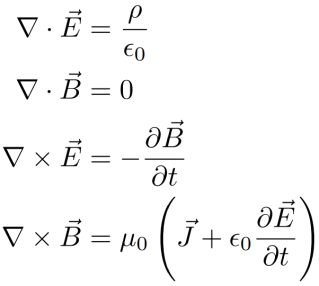
Vector Calculus and Electromagnetism

Vector calculus is an extremely interesting and important branch of math with very relevant applications in physics. Specifically, vector calculus is the language in which (classical) electromagnetism is written. It is fascinating to me that Maxwell’s equations can so succinctly and elegantly express so many phenomena, from electric and magnetic interactions to light (electromagnetic waves). One popular formulation of Maxwell’s equations is the following:

So what does this all mean? Let’s break it down, arduously and tediously, from the nitty-gritty of the vector calculus requisite for understanding the elegance of these equations.

Note: I presume basic knowledge of calculus in this post. Obviously, this is not meant to be a substitute for a more rigorous foundation with more computational practice.

Part 1: Vectors and Functions with Vectors

First, let’s talk about vectors. Specifically, let’s handle them in an intuitive sense. There are precise definitions for vectors and vector fields provided by linear algebra, and vectors/vector fields have been subjected to many degrees of abstraction and generalization in mathematics, but let’s just take for granted that vectors represent these sorts of “arrows” in space.

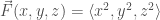
Vectors have a “magnitude,” or length, and a direction. A vector can be expressed in terms of these two properties:

Here,  is the length of the vector and is a vector in the direction of with a length of (note that the “hat” notation is substandard in mathematics, although it is quite standard in physics).

Vectors can be added—to add two vectors and , just align the tip of to the tail of . The resulting vector is the vector with its tail at the tail of and its head at the head of (adding “tip-to-tail”):

It is important to establish the difference between scalar fields and vector fields in (in a sense, all “places” that can be represented by three real numbers, which pretty much means 3D space). Both of these concepts just represent functions. Recall that a function is roughly an object that takes in an input and returns an output. A function (read: a function which takes real numbers and outputs real numbers) could look like this:

Such functions are the subject of much discussion in early math classes, but this idea can be generalized. A function can also take in multiple inputs or output vectors, which can be expressed as -tuples (lists of numbers). When a function takes in multiple inputs, it is often regarded as taking as input a vector. The objects of interest here are scalar fields and vector fields in . A scalar field in  is a function —it takes in three real numbers (basically, a vector) and outputs a single number. For example, a scalar field might be:

It is called a scalar field because it outputs a scalar. This can be thought of as an assignment of a number to every point in space.

In contrast, a vector field in is a function —it takes in a vector and outputs another vector. An example of this might be:

Analogously to scalar fields, vector fields can be thought of as assigning a vector (read: arrow) to every point in space.

Part 2: Vector Multiplication

There are several different processes that can be described as “vector multiplication.” First, there is scalar multiplication. There are also ways to “multiply” two vectors together. In , there are two products of note: the dot product and the cross product.

Scalar Multiplication

Probably the easiest of these to understand is multiplication by a scalar, or a number. Basically, when a vector is multiplied by a number, its length gets multiplied by that number:

The Dot Product

The dot product is an operator between two vectors that returns a scalar. Specifically, a dot product takes the first vector’s “component” along the direction of the second vector. It then takes the length of that component and multiplies it by the length of the second vector:

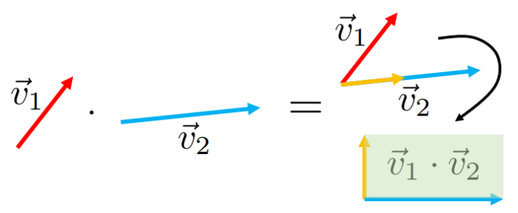
It turns out, computationally, that, for two vectors given by

the dot product in between the two is given by

Note that this means that the dot product commutes (i.e. ).

The critical observation to make here is that the dot product is at its maximum when the two vectors are pointing in the same direction, at its minimum when the two vectors are antiparallel (pointing in opposite directions), and zero when the two vectors are perpendicular. This makes it a useful tool for defining the concept of vectors being parallel and perpendicular without making reference to intuitive geometric notions of these concepts.

The Cross Product

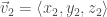
The cross product, on the other hand, is an operator between two vectors that returns another vector. Specifically, it takes the length of the component of the first vector in the direction perpendicular to the direction of the second vector. It then returns a vector with the length of that first component multiplied by the length of the second vector. The direction of the cross product is given by the right-hand rule (by convention), but the important thing is that the cross product will return a vector that is always perpendicular to the input vectors (note that, also by convention, the vector, the vector with zero length, is perpendicular to all vectors).

Since there are (in general) two different directions that a vector can point to be perpendicular to two other arbitrary vectors, the right-hand rule disambiguates the direction that the cross product actually points (as the name suggests, the usage of the right hand here is critical):

The cross product is a useful way of generating a vector that is guaranteed to be perpendicular to two other vectors. Interestingly, unlike the dot product, the cross product is not generalizable to arbitrary numbers of dimensions while keeping the output a vector (a sort of “generalization” called the wedge product exists, but it outputs an object called a “bivector,” not a vector).

All three of these “vector products” will be used to explain the different types of derivatives in by analogy.

Part 3: Vector Derivatives

In functions , derivatives can be defined between the input and output variable. Namely, for a function like

a derivative for the function in terms of can be written:

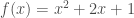
In functions that take more than one variable as input, however, this gets a little bit more tricky, and we will tend to define “partial derivatives” for such functions. Partial derivatives are always with respect to one variable, and, in the computation of a partial derivative, any other variables are treated as constants. The reason why these derivatives are “partial” is because knowing a partial derivative and an initial condition is not sufficient for determining what a function looks like, since it does not account for all the ways that a function could vary. Consider the following function:

Noting the slightly different “” notation, the following partial derivatives can be defined:

As the method for computing partial derivatives suggests, partial derivatives represent the rate of change of a function when one variable is allowed to vary and the others are held constant. This represents a sort of “slice” of the function.

With this out of the way, we can define three types of derivatives in : the gradient, curl, and divergence.

The Gradient

It is perhaps easiest to explain the first of these, the gradient, in terms of scalar fields which take in two numbers instead of three, since the sum of the input and output dimensions here is , which is the most number of dimensions that can easily be visualized at once. The gradient of a scalar field can be written as or (where the symbol is pronounced “del” or “nabla”).

Importantly, the gradient is a derivative of scalar fields. There is no “gradient of a vector field” (update 07/31/2017 — It has been pointed out to me recently that such a concept exists, but, importantly, this gradient would not be a vector but a more general object called a tensor). Broadly, the gradient represents the direction of fastest ascent of a function.

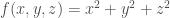
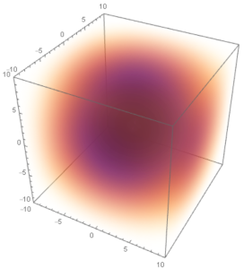
Consider the following function:

A plot of might look something like this:

The gradient of , plotted over this surface, might look something like this:

Note that, while I have aligned the vectors of the gradient over the original surface, the actual vector field is still a two-dimensional vector field. Its direction represents the direction of fastest ascent (the direction in which the function increases the fastest), and its magnitude represents the slope of the function in the direction of fastest increase.

The gradient can be represented as a vector of the multiple partial derivatives. In , this can be written as:

For a three-dimensional vector field, this is easily extendable:

Note that the gradient can be integrated over along a curve in order to find the value of a scalar function given an initial condition. Note the relationship here between a quantity—the difference between a start and end point along a curve—and some quantity that lies in between these boundary points, a quantity called the gradient. While this seems strange to point out specifically here, it is relevant to see this concept in analogy while thinking about curl and divergence.

Curl

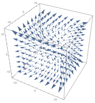
The curl, in contrast to the gradient, is a derivative of vector fields, and the curl itself is a vector field. For a vector field , it can be written as or . Let’s consider the following vector field:

Below is a plot of :

looks like this:

Of course, we haven’t really discussed what the curl actually represents. Doing so, and defining it a little more precisely, will allow us to “derive” an intuitive expression for curl. We can talk about a concept called circulation. This first requires that we talk about line integrals.

Suppose there is some oriented curve in (this curve is in three-dimensional space but is, itself, a one-dimensional object). By oriented, I mean that there is a certain “direction” that we call positive. Then we can define the line integral  of the vector field along the curve as given by

where

This expression might be difficult to unpack, but, basically, the idea is to break the loop into very small segments , take the dot product of each small segment with the value of the vector field at that point along the curve, and sum up all the dot products along the curve.

The circulation is exactly this concept, but with closed curve. The circulation of a vector field along a closed curve is given by

where the symbol just emphasizes that the integral is along a closed path.

Closed curves are just curves where the beginning and end of the curve are the same point. In other words, as the name suggests, they are “closed.” Suppose we have a closed curve that looks like this:

You can split into two separate closed curves and :

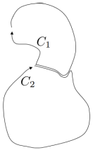
The circulation along is actually just the sum of the circulations along and . The reason why is that the parts of and comprise the sections of the curves that overlap with , and the other parts of and , where the curves overlap, run in opposite directions, so the line integrals along those portions cancel out.

A consequence of this is that we can split the curve into many, many very small curves, and the sum of the circulation about each little curve is the circulation about .

Of course, the circulation of a curve will, generally speaking, go down as the curve itself goes down. This means that it benefits us to divide this quantity by the area bounded by the curve. Curl can be thought of the circulation per area of a vector field. However, because there are three dimensions, there are three different ways that the vector field can circulate. This means that curl is a vector.

A more formal definition of curl by Khan Academy can be found here.

Suppose that there is a rectangle-shaped oriented curve that looks like this:

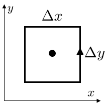
We can approximate the circulation from each side of the rectangle as the length of that side multiplied by the component of the vector field in that direction (with the orientation of the curve accounted for). Defining the vector field as 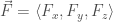at the center of the rectangle, we can use linear approximations to estimate the value of the vector field at each side of the rectangle.

Note that we define the direction of a rotation as the vector normal to (read: perpendicular to) the surface bounded by the curve along which there is circulation. In particular, we apply the right-hand rule here; if you stood on the curve and walked around it in the direction of its orientation, the rotation is defined as pointing in the direction such that your head would point if turning to the left faces you towards the surface (if this is confusing, it’s not essential to understanding curl conceptually, although this convention is certainly important for doing actual computations). This gives us the “direction” of the curl.

The circulation about this rectangle then becomes

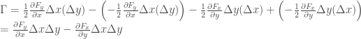
Dividing this by the area gives an approximation for the curl:

As the rectangle is made smaller and smaller in both directions, this approximation to the curl actually becomes exact, and we are left with the value of the curl in the -direction. Doing this for the – and -directions will yield the following formulation for curl in Cartesian coordinates:

An interesting note is that the identity 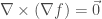(the curl of any gradient is the zero vector). An intuitive way of visualizing this is that the gradient represents a sort of increase in altitude that one experiences when walking around the “surface” created by a scalar field. If it were not true that , you would be able to walk in a circle and somehow end up at a higher altitude, which is nonsensical.

Divergence

The last derivative of interest to us is the divergence. Like the curl, the divergence is a derivative that applies to vector fields. However, unlike the curl, the divergence is a scalar-valued operator; rather than assigning a vector to every part of a vector field, it assigns a scalar. The divergence is written as or .

Divergence is, essentially, the tendency of a vector field to “diverge” from a point. That is, divergence captures the extent to which a vector field flows outward from a point.

The vector field in the previous section about curl has a divergence that looks like this:

Instead of circulation, now, the quantity of interest to us is called flux. Suppose we have an oriented surface . By oriented, I mean that one direction through the surface is considered positive, and the reverse direction through the surface is considered negative. Then the flux through that surface is, intuitively, the number of “lines” that pierce the surface. More precisely, we can break up the surface into a bunch of little surfaces. Then, we can multiply the magnitude of the component of the vector perpendicular to the surface by the area of that tiny surface. Finally, we can sum up all of these quantities to obtain the flux. If is the flux of the vector field through the surface , then

where  is a tiny oriented surface.

Just as there are closed curves, there are also such things as closed surfaces, which are surfaces that close in on themselves (like a sphere). A closed surface could look this:

We can split the volume bounded by into two volumes and consider the surfaces that bound these new volumes, which we can call and :

Just as we needed to apply some sort of convention when considering circulation (i.e. the right-hand rule), by convention, flux is positive when the number of “lines” exiting a surface exceeds the number of lines entering it. Consequentially, it is negative when there are more “lines” entering the surface than exiting it.

Note that the flux through is just the sum of the fluxes through and . This is because the parts of the new surfaces that don’t overlap with the original surface overlap with each other, but are oriented in opposite directions. Any “lines” that pass through the overlapping surface leave one of the surfaces but enter the other one. This leaves us with the flux through .

This means that, just as with curl, where we were able to split up the area into many tiny areas, we are now able to split the volume bounded by our surface into many tiny volumes with their own bounding surfaces. Once again, since the surface area will go down as the volumes are reduced in a reasonable fashion, the flux will decrease the more the volume is split up. This means that it is useful for us to divide this flux by volume. This flux per volume is what we mean when we refer to as the “divergence” of a vector field.

Khan Academy formally defines divergence here, and a two-dimensional analogous version is defined here.

Just as with curl, we can apply linear approximations in order to “derive” some sort of formulation for divergence in Cartesian coordinates. First, we imagine a cube-shaped closed surface:

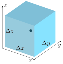
We can then calculate an approximation for the flux by taking the component of the vector field pointing outward from the cube at the center of each face and multiplying it by the area of that face, and summing over every face. This yields the following expression for flux out of this surface:

We can then calculate the flux per volume by dividing by the volume of the cube :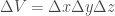

As the cube-shaped surface is reduced in size, this formulation becomes exact, and we have

Before, I noted that . Interestingly, the identity (the divergence of any curl is zero) also holds. While the intuition for this is less clear, curls can be thought of as representing “axes of spin” of rotation in a vector field, and it would be strange if such axes could come out of existence at a defined point. It seems comforting that mathematics agrees that axes of spin can’t just come out of nowhere.

These three types of derivatives can be understood by analogy with a stream. The gradient is like dropping a leaf into the water and seeing which direction it gets pushed, which is a characteristic of the pressure of the water at every given point. The curl is like putting a little pinwheel into the water, and seeing how quickly the pinwheel can be made to turn in a given time for every direction the pinwheel is oriented. Finally, the divergence is like putting a closed net into the stream and seeing how much water flows out of the net.

The Operator

We used the symbol in defining the notation that we used for the gradient, curl, and divergence, but we didn’t really discuss the significance of such notation. Indeed, it is no coincidence that the gradient’s notation looks like the scalar multiplication between  and , the curl’s notation the cross product between  and , and the divergence’s notation the dot product between  and .

Indeed, we can define the operator as the following:

It may seem a bit peculiar to define a sort of “vector” object with derivatives without functions, and it might seem a bit weirder when we accept that applying an operator amounts to right-multiplying an operator by a function, but the notation is evocative enough to overlook these concerns. Once we define the symbol as above, the gradient really becomes the product between the and the scalar field :

The curl really does become the cross product between the and the scalar field :

Again, the divergence really does become the dot product between the and the scalar field :

Somehow, the fact that this notation is so evocative of the calculation of these quantities in Cartesian coordinates lends more elegance to these concepts.

Part 4: Stokes’s Theorem and Vector Calculus

Perhaps the most foundational theorem in calculus (a status conveyed quite explicitly by its name) is the fundamental theorem of calculus. While the fundamental theorem of calculus makes two statements, we will concern ourselves with the following:

The Fundamental Theorem of Calculus is particularly interesting because it relates the summed over quantity of a function (namely, the derivative) to a property of the boundary of the interval being examined (the difference between the function at the upper and lower bounds of integration. Note that the particular values of the function cannot be gleaned by just knowing the derivative, only this aforementioned property of the boundary. Nevertheless, by applying initial conditions and constraints, the function can be found anyway.

There exists an analogous theorem for the gradient, called the fundamental theorem of line integrals, which states the following:

A side note: it becomes clearer after examining this theorem why vector fields that curl cannot be gradients (i.e. they are not “conservative”). This is because, for a closed curve line integral, the start point and endpoint of the scalar field should be the same, so the line integral should evaluate to zero. If it doesn’t, we are forced to conclude that there is no scalar field such that our vector field is the gradient of .

I would like to point out that, once again, the fundamental theorem of line integrals relates the gradient, a property of a function at every point, with the difference between a boundary property, the difference between the start and endpoint of a line (a domain being integrated over). Again, the theorem does not uniquely determine what the values of the function are, but only the difference between the function’s value at the boundary of the interval.

Of course, this can be extended further: the Kelvin-Stokes theorem (often just called Stokes’s theorem, although this is technically ambiguous) is a very similar theorem for curl. It states the following:

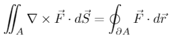
for some surface and its boundary curve (note that the “” symbol referring to the boundary of a surface is considered substandard in many circles). Note that the “double integral” symbol just reflects the fact that a surface, rather than a curve, is being integrated over.

Now, a continuous property of a function, the curl on a surface, is being related to a boundary property (once again), this time the circulation about the boundary curve of the surface. Once again, this information does not uniquely decide what the vector field is, but only this “boundary property.”

Finally, unsurprisingly now perhaps, the divergence theorem (also known as Gauss’s theorem) does the same thing for divergence. In particular, it states that

where is an infinitesimally small element of volume, is a volume, and is the boundary surface around that volume, and where the “”

Now, the fact that the divergence of a curl being zero is elucidated somewhat. Instead of considering a closed surface, we can consider a surface with a very tiny hole, and the boundary of that hole (which is also the boundary of the surface) will have a very small circulation. That means that, by the Kelvin-Stokes theorem, there is also a very small flux (of the curl) through the surface. As we make the hole smaller and smaller, we can imagine the surface “closing” (although this intuitive “proof,” it should be noted, is not rigorous at all) into a closed surface, the flux through which should now be zero.

Once again, the divergence theorem relates a property within a domain, the divergence in a volume, with a boundary property, the flux, which, again, doesn’t, without boundary conditions or constraints, uniquely determine what the vector field actually is.

If I haven’t beaten to death this idea of a relationship between the derivative in a domain and some boundary property of that domain, perhaps we can view this result in a way that makes us realize that it couldn’t have been any other way. After all, we define the derivative to be something like the “change of a function over an interval” (read: difference in the value of a function at the high and low ends of an interval), the gradient to be a vector conveying the same thing for functions of more than one variable, the curl as the circulation per area, and the divergence as the flux per volume. Of course it would be the case that, if we sum over these quantities multiplied by the denominator quantity, we should get the numerator quantity.

It also illustrates a deeper connection that is elegantly expressed in Stokes’s theorem, a famous result in differential geometry:

This is the ultimate expression of the relationship between a quantity on the surface (read: boundary) of a manifold and its derivative over the entire manifold. While not necessary to know about in order to have a rewarding understanding of electromagnetism (which this post is ultimately aiming at, believe it or not), I felt that Stokes’s theorem (in generality) represents an extremely beautiful aspect of the underlying mathematics.

Part 5: Maxwell’s Equations

Now that we’re finally done with the ideas behind basic vector calculus (which are beautiful in and of themselves), we can start to explore the meaning of Maxwell’s equations. Again, they are the following:

First, it is important to note that Maxwell’s equations relate the electric () and magnetic () fields to charge density () and current density (), with reference to the vacuum permittivity () and permeability () constants. In particular, it defines the divergence and curl the electric and magnetic vector fields in terms of their time derivatives as well as charge and current density. Let’s explore these equations one by one.

Note: Computationally, it is often easier to treat Maxwell’s equations in integral form. The integral formulation is equivalent to the differential formulation above (by the Kelvin-Stokes and Divergence theorems), but I find the differential formulation to be vastly more elegant. While Maxwell’s equations claim general truth, they are often only computationally useful when there is exploitable symmetry (e.g. it can be known a priori that the electric/magnetic field must be uniform on a surface/along a curve, etc.).

Gauss’s Law (for electric fields)

The first of Maxwell’s equations, Gauss’s law (for electric fields), relates the divergence of an electric field to the charge density. Its statement is the following:

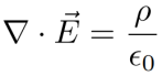
The equation is straightforward after understanding the concept of divergence. Basically, wherever the electric field “diverges,” that is, wherever more electric field leaves a point than enters it, there is positive charge, and wherever more electric field enters a point and leave sit, there is negative charge.

Within a constant multiplier (which depends on the system of units), wherever there is charge (density), there is electric field—charge density is essentially the divergence of electric field.

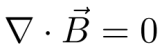
Gauss’s Law for magnetism

The second equation, or Gauss’s law for magnetism, states an important truth about magnetic fields. In particular, it states that

Faraday’s Law

Basically, this means, whatever the magnetic field is, it does not diverge. There is no such thing as “magnetic charge.” There isn’t any particular reason why magnetic charge (and thus magnetic current) doesn’t exist. In fact, magnetic monopoles are predicted by some theories, and cosmologists often accept inflationary theory as the reason why we don’t see any. However, consistent formulations of Maxwell’s equation taking into account theoretical magnetic charges (“monopoles”) do exist, and Gauss’s law for magnetism thus represents an empirical observation about the nature of magnetism.

The third equation, Faraday’s law, lays the groundwork for how electricity is harnessed for energy. It relates the curl of the electric field with magnetic fields:

In essence, it states that, the more quickly magnetic field increases in a certain direction, the more strongly the electric field will curl against it (the “against” bit of this statement also has its own name, Lenz’s law). Significantly, since is related to voltage, moving a magnet will create electric fields (and thus voltage), and this has its applications in energy generation.

It is also interesting to note that, when there is a steady (non-changing) magnetic field, the electric field does not curl.

Ampère’s Law (with Maxwell’s displacement current contribution)

The fourth, and final equation is Ampère’s law (specifically, with a “displacement current” modification). The statement is as follows:

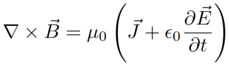
Just as the electric field diverges from charge density, magnetic field curls around current density. In addition, magnetic field will also curl around a changing electric field (this requirement can be motivated by the fact that circuits with capacitors can have current that flows for a time even when the physical charges can’t move across a physical gap, and we want our equations to be consistent).

To be clear, any expressions for electric and magnetic fields that follow Maxwell’s equations should be possible in principle (although I’m not trying to assert the possibility of actual infinite sheets of charge, as any student of electromagnetism might humorously point out).

The Lorentz Force Law

The final equation needed to describe electromagnetism is the Lorentz force law:

But wait? We have already defined both the curls and the divergences of the electric and magnetic fields. Surely we have constrained them enough to get quite specific about what kinds of electric fields and magnetic fields are possible, and that is true.

However, the more salient question for the observant is more fundamental than that: what even are electric and magnetic fields?

It is important to remember that electric and magnetic fields are really proxies for describing real things that happen. What good would defining electric and magnetic fields even be if they had no effect on motion?

Indeed, the Lorentz force law links the electric and magnetic fields to force (as its name hints). In particular, the force contribution due to an electric field points either in the same or opposite direction as the electric field, and the force contribution due to a magnetic field points in the direction given by the , where is the velocity vector of the charge. The magnitude of the force from the electric field is proportional to the absolute value of the charge and the magnitude of the electric field, and the magnitude of the force from the magnetic field is proportional to the absolute value of the charge, the magnitude of the velocity vector, the magnitude of the magnetic field, and the angle between the velocity vector and magnetic field.

But where does gradient come in?

After all this discussion about electromagnetism, we still haven’t handled the gradient. Actually, the gradient still has meaning in electromagnetism. In particular, if is the electric potential (in circuits, often also called the voltage), then

Update 07/31/2017 — The above is only true in electrostatics (i.e. there are no moving charges). When there are moving charges, this instead becomes .

While it seems odd at first that we want to define the concept of electric potential, we can first make reference to the fact that electric fields do not curl in the absence of a changing magnetic field. This means that the electric field is allowed to be the gradient of a function, so we are guaranteed that a exists, so long as the magnetic field is steady. We define such a concept because it is often easier to handle a scalar field like rather than a vector field like . If the voltage is the landscape, a field of “hills” and “valleys,” the electric field points in the direction of greatest descent (note the negative sign). In this context, the electric field represents which direction a charge will “roll down,” and how quickly that will happen.

A similar concept exists for magnetic fields. Specifically, the magnetic (vector) potential satisfies a similar relationship with magnetic field. These quantities are related by curl, rather than the gradient:

Part 6: Review and Conclusion

I went over a lot of stuff in this post that can be summarized very broadly in the following, slightly busy flow chart:

Electromagnetism is an incredibly insightful theory, representing the union of two forces historically regarded as very different, yet two different facets of the same coin. In addition, the theory motivated Einstein to formulate his theory of special relativity, which led to his formulation of general relativity (in fact, electric and magnetic fields necessitate each other by special relativity, but that’s for another time). Electromagnetism also predicts the speed of light, allowing for light as an electromagnetic wave.

While contemporary theories like quantum electrodynamics and special relativity more generally describe and contextualize the phenomena examined by classical electromagnetism, classical electromagnetism nevertheless represents a stunningly elegant as well as pragmatic representation of one of the fundamental forces governing the evolution of the universe.

A pdf version of the Mathematica notebook used to make the images used in describing the vector derivatives can be found here. Notable textbooks on vector calculus by Stewart and on electromagnetism by Purcell and Griffiths provide a much more thorough examination of these topics.

Update 07/31/2017 — Someone noticed that the formulation of Maxwell’s equations I refer to are the “microscopic” version of Maxwell’s equations. Specifically, they pointed out that another formulation exists which accounts for a varying permittivity () and permeability () by defining two new fields, and . While the macroscopic formulation is oftentimes much more useful, the microscopic version, in principle, is more often “true,” although teasing out “macroscopic” consequences is generally inconvenient (e.g. the fact that light slows down when passing through matter).