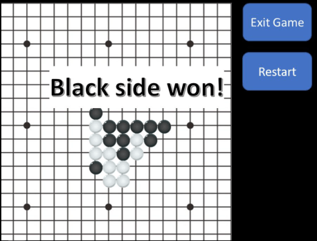
Recently, one of my good friends was telling me about her final project in an introductory programming class for physics. She and her partner created a game in the style of tic-tac-toe, with opposing sides, black and white, placing markers on a grid until one side creates a line of five pieces in a row:

Interested, I asked to look into the code.

As I expected, the lines that checked whether a player had achieved a five-in-a-row was a verbose series of nested for-loops checking a plethora of cases. While they often seem like a natural course of action, in many settings they are often unwieldy and slower than desirable. Luckily for my friend, the code ran quite quickly, but I thought about whether there was a faster way.

Luckily, there are some very common modules in Python which provide alternatives to for-loops in many cases, one of which is NumPy (I recognize that it’s probably intended to be pronounced “Num-Pai,” but I find the pronunciation “Num-Pee” more affectionate).

NumPy handles data in a way that stock Python cannot by utilizing objects called arrays. While, at first, arrays appear to serve a very similar function as lists, they are actually quite different. You can see this immediately when you try and add two lists together, and when you add two arrays together:

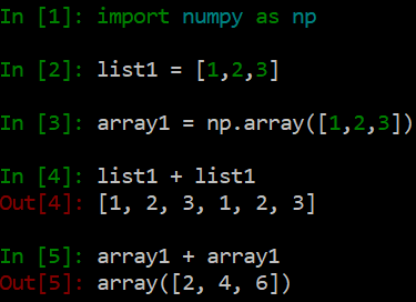
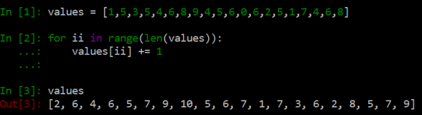
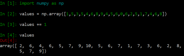
While adding lists simply appends the second list to the end of the first, adding arrays is element-wise, adding each element together one-by-one, but all at once. The first advantage is that NumPy is more succinct than for-loops, although this is, of course, just aesthetic. Suppose I wanted to add 1 to every number in a list. With for-loops, I would be writing

whereas the NumPy array route is more direct:

However, while aesthetics and intuition definitely matter, what really gives NumPy its power is the efficiency at which it can process operations like this. I wasn’t able to notice a difference between these last two examples, but suppose, instead of working with twenty elements, we were working with one million? There is a massive speedup! Using for-loops, adding 1 to each element in a list of one million numbers took me 293 ms. Doing the same exact operation to the same exact numbers with NumPy arrays only took 2 ms. That’s a speedup of almost 150 times!

Now, 293 ms is still not bad, but we have to keep it within the context that usually, in data analysis, there isn’t utility in adding 1 to a million random numbers. As a test case, it demonstrates how fast the speedup is. After having waited for my computer for twenty or thirty minutes to do many simple operations to large numbers of numbers, I have gained a newfound appreciation of efficient data manipulation.

However, in this case, NumPy didn’t provide all the tools necessary to execute this speed-processing vision sufficiently.

Convolutions

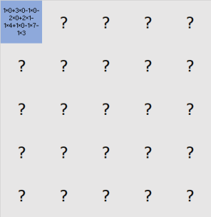
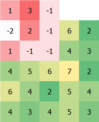
In this context, convolutions are operations that take two arrays of numbers and return another array of numbers that quantifies, in some way, how much the arrays overlap. Another way of thinking about this is that a convolution takes an array and adds to each point the value of its neighbors, modulated by (possibly negative) weights. For example, if we start with the following array

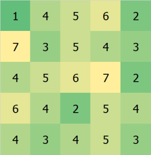
and convolve it with the following set of weights (also called a “kernel”)

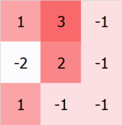
we first line up the kernel with the top left pixel:

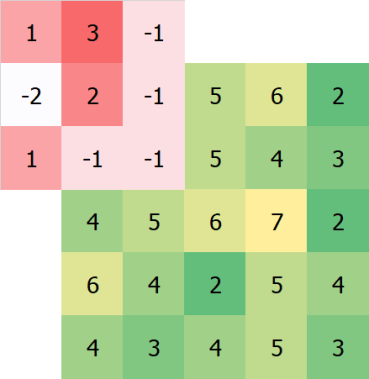
We then multiply the overlapping numbers together, and then add the results all together. We then assign that number to the top-left pixel:

Then, line up the kernel on the second pixel:

Rinse and repeat, until we have:

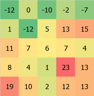
Voilà, the convolution.

The convolution also often appears as a one-dimensional operation as well as a continuous operation between two functions, as well as through a very similar but slightly different operation called the cross-correlation, which has uses in astronomy and other fields. The convolution is also central to a method of machine learning in structures called convolutional neural networks, which can be made to do pretty amazing things.

Note that, if you just picked a kernel with a 1 in the middle and 0s elsewhere, you would just get the same grid of numbers (which can represent an image) back. If we “dampen” this so-called Dirac delta kernel so that it is more spread out (i.e., with a large number in the center and numbers that decrease with distance from the center, all adding up to 1), then we get a Gaussian kernel, which is responsible for Gaussian blurs and provides a very easy-to-understand way of blurring an image (to see why this works, remember that blurring essentially amounts to smudging a pixel with its neighbors, which is basically what is going on here). Finally, if you take a Gaussian kernel and subtract a Dirac delta kernel, you have the basis for a method called unsharp masking, which is what you do when you want to find the edges in an image (and possibly enhance them).

Clearly, convolutions are pretty cool.

Because convolutions are very important to signal processing, its appropriate that Scipy‘s signal commands include a 2D convolution function (scipy.signal.convolve2d).

Back to our original problem of how to check if there is a five-in-a-row, we can apply the following kernels:

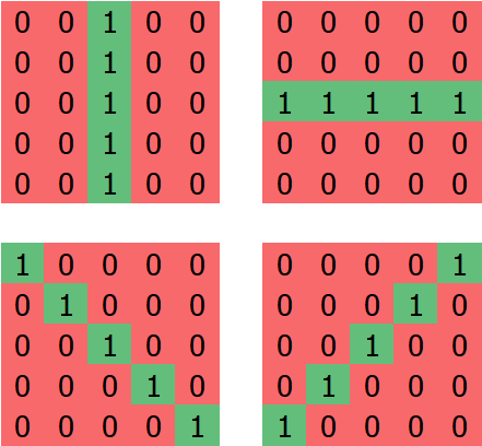
Together, these kernels will check if there is a five-in-a-row anywhere on the board. As a bonus, if we choose to represent the game as a grid where white is positive and black is negative, the convolution filters will even be able to tell which side won (although this should be pretty obvious since the game is turn-based). If a (positive or negative) 5 appears anywhere on any of the results of these convolutions, we know that the game is over.

Below, on the left, I generated a grid of black and white squares. On the right, the black squares represent all pixels on the left side which are the center of some five-in-a-row pattern of black squares:

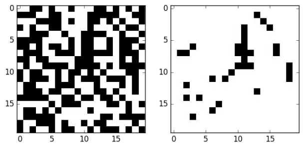
How quickly did this speed up my friend’s game? Actually, the improvement wasn’t too great, only on the order of milliseconds or so, but an improvement nonetheless. What else can we do?

The Game of Life

The Game of Life is the brainchild of John Conway. As a cellular automaton, the idea is that we start with a grid with spaces that are either “alive” or “dead.” In order for a dead space to become alive (or “born”), exactly three out of eight of its neighbors must be alive. In order for a space that is already alive to stay alive, it must have either exactly two or exactly three neighbors alive. Otherwise, it “dies” of either “loneliness” or “overcrowding.”

In other words, the rule set is B3/S23 (for “birth” with 3 neighbors and “survival” with 2 or 3 neighbors). The rule set can be changed with many other weird behaviors. There are, of course, apps that let you explore these behaviors. Here is one of my favorites.

In addition, if you want your cellular automaton to actually care which of its neighbors are alive (as opposed to just counting them), you can get even more interesting structures with even more crazy rules.

These decisions are made step-wise, all at once. Interestingly, while the rules of this “game” are extremely simple, there is a lot of very complex behavior. I’m not going to get into it here, people have been able to construct programmable computers, digital clocks, and even the Game of Life within the Game of Life. As a student of physics, it’s very elegant that such simple rules can cause such a spectrum of interesting structures, and it lends hope to an elegant structure all the way down in the real world.

Anyway, to make the Game of Life in Python, I used the following kernel:

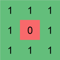
After convolving the current state of the board with this kernel, each point on the grid is assigned the number of neighbors it has. Together with the current state of the board, it becomes very easy to compute the next state of the Game of Life. Using these packages and some magic from Matplotlib, I was able to create the Game of Life in Python:

Can we have even more fun?

The input and output grids for the convolution were all discrete, each space on the grid represented by either a 0 (for dead) or 1 (for alive). However, I wondered if I could make these states take values continuously between 0 and 1. What would this look like?

In order to make the rules work, I created a map of desired outcomes as a function of current state and number of neighbors. I then interpolated over these states linearly to obtain: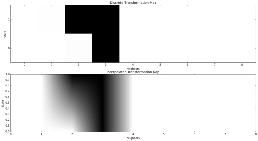

Generating a grid of random numbers as an initial state, my curiosity was thus satisfied:

I didn’t really get into the behavior of this thing. It seems quite chaotic and I’m not sure any stable structures can form in it. I do know that, if I initialize the state using only 0s and 1s, it will behave exactly like the Game of Life proper; this isn’t really surprising.

Of course, people have done even cooler things with the Game of Life. For example, there have been even more sophisticated continuous versions, as well as a literal game based off of the Game of Life. Someone has even taken the idea of convolutions and run with it, creating a convolutional neural network that “learned” the rules of the Game of Life. Pretty cool stuff.

What else can be done with this stuff? Who knows? Even more fun to be had.