Linear Algebra and Quantum Mechanics

When I was younger, I would occasionally hear about higher math classes that one was able to take. To me, then a naïve high schooler, AP Calculus represented an attainable pinnacle of mathematical knowledge beyond which lie a plethora of weird maths to explore. I had heard of multivariable calculus, which sounded like more of the same with more letters, differential equations, which was just calculus with more tricky problems, and so on and so forth.

However one, linear algebra, seemed like a mystery. It’s name evoked, to me, the kinds of problems done in middle school where I was painstakingly asked to grind through systems of three equations to find $x$ , $y$ , and $z$ . Sure, I thought, maybe there’s a use for solving ever bigger systems of equations of ever increasing complexity with bigger and better techniques. But, if multivariable and diff-E.Q. were “more of the same,” jumping back to middle school lines and planes was definitely going be a bore.

Spoiler alert: It wasn’t, and, while related, linear algebra really isn’t about that stuff. It’s actually about a lot of other, cooler stuff, including really cool stuff like quantum mechanics.

Note: This is just a primer on linear algebra. I introduce the axioms, and then paint over the subject with a broad brush that isn’t meant to be comprehensive. Quantum mechanics is inseparable from linear algebra, so I try to get to the meat of linear algebra while not glossing over too much. At the same time, this obviously shouldn’t be taken as a substitute for a more rigorous treatment of linear algebra.

Part 1: The Abstract

All throughout grade school, I was decent at math, but I was lacking one key piece of mathematical maturity: I relied on intuition to do math, and struggled when that failed. When looking at a function, I would imagine the graph. When doing trigonometry, I would imagine triangles. I did calculus by imagining the summing up of little pieces rather than by working through the more rigorous sea of Riemann sums and so on.

While this isn’t really all that bad for most everyday purposes, it certainly becomes a problem when trying to do upper level math. It took a long while for me to realize that math isn’t so much about describing physical things (which is the domain of physics), but more about asking the question what if? about increasingly abstract concepts and working out what would happen. It’s about assuming certain statements, called axioms, and deriving results, called theorems in order to understand what an object that followed said axioms would behave like.

For the reader who is new to such thinking, I caution you: use your intuition, but don’t get caught up in what “all this stuff is, really?” A lot of it is going to sound vague, but that sort of answers the question of what this stuff is about, which is, as it turns out, a whole lot of stuff.

For this introduction to linear algebra, I will use some mathematical notation in order to ease in the more compact notation for what I’m saying. However, I will be sure to explain what I’m saying in normal well-adjusted human language in close proximity when I do so. I also won’t bother proving every single statement, but will be sure to prove some of the more important ones.

This introduction is about the theory of vector spaces and linear transformations, rather than the computational, matrix-math aspect of linear algebra. Admittedly, that’s leaving a lot out, but hopefully this is a helpful overview of a summary course on the subject.

Part 2: A Theory of Vector Spaces

Definition: A field is a set $F$ which is a generalized notion of numbers with some nice properties. I won’t really go into what defines them precisely since it isn’t all that important for our purposes (those defining axioms can be found here). However, some examples of fields are below:

$\mathbb{Q}$ : The rational numbers, numbers which can be expressed as a fraction of integers
$\mathbb{R}$ : The real numbers, numbers which each represent a point on a number line
$\mathbb{C}$ : The complex numbers, a set of numbers big enough so that every polynomial equation as a solution in $\mathbb{C}$ (for this, we introduce a number $i$ such that $i^2=-1$. Don’t think too hard about how this is possible, this is what I mean by asking what if?)
Finite fields like $Z_2$ , $Z_3$ , $Z_5$ , etc. These are less intuitively but still technically fields. While they are fun and interesting in their own right, I will ignore them since they won’t be all that interesting for the end goal here, which is understanding how linear algebra is related to quantum mechanics.

I will commonly refer to objects in a field as numbers or scalars.

Definition: A vector space $V$ over a field $F$ is a set of objects, called vectors. This set has two binary operations:

$+: V\times V\rightarrow V$ (vector addition). These symbols just mean that there is an operation called $+$ which takes two vectors which are in the vector space $V$ and returns another object which is also in $V$ . It is important that two vectors in $V$ , when added together, give another vector which is also in $V$ . This is called closure, and vector spaces are said to be closed under vector addition.
$\cdot: F\times V\rightarrow V$ (scalar multiplication). This is an operation that takes in a number from the field $F$ (which we are leaving general at the moment) and a vector in $V$ and returns a vector also in $V$ . Scalar multiplication also obeys closure, so we have that vector spaces are closed under scalar multiplication. I will often omit the $\cdot$ symbol and just write the scalar next to the vector. For example,

In addition, in order for $V$ to be a vector space, it must obey the following axioms:

Vector Addition Axioms:

$x+y=y+x\forall x,y\in V$ . For any two vectors in $V$ , I must be able to add them in either order and get the same thing. This is called commutativity, and may be familiar from middle school when learning about number addition.
$x+(y+z)=(x+y)+z\forall x,y,z\in V$ . For any three vectors in $V$ called $x$ , $y$ , and $z$ , if I add $x$ and $y$ together, and then add $z$ , that is equivalent to adding $x$ to the sum of $y$ and $z$ . This is called associativity, which should also be familiar.
$\exists w\in V$ s.t. (“such that”) $x+w=x\forall x\in V$ . There is a special object, which I’m calling $w$ for now such that, when I add it to another object, the result is always that other object. From now on, I will call this vector $0$ . I will justify why I can do so in a bit. This is saying that there is a zero vector, also called an additive identity.
$\forall x\in V\exists y\in V$ s.t. $x + y = 0$ . This is the statement that, for every vector, there is some other vector which, when added to the first vector, gives $0$ . I called these vectors $x$ and $y$ , respectively, but, from now on, instead of saying $y$ , I will say $-x$ . I will justify this later as well. This is the notion of additive inverses and basically tells me that I am allowed to do subtraction (which is just glorified addition involving inverses).

Scalar Multiplication Axioms:

$1x=x\forall x\in V$ . The $1$ on the left is the $1$ scalar (in $F$ ). If I multiply a vector by the number $1$ , the vector is left unchanged.
$a(bx)=(ab)x\forall a,b\in F, x\in V$ . If I multiply a vector $x$ by a number $a$ and then multiply the result by another number $b$ , I will get the same thing as if I multiplied those numbers together to get $ab$ and then multiplied the result by the vector $x$ .

Distributive Axioms:

$a(x+y)=ax+ay\forall a\in F, x,y\in V$ . Scalar multiplication distributes over vector addition.
$(a+b)x=ax+bx\forall a,b\in F, x\in V$ . Scalar multiplication distributes over scalar addition.

These two axioms are the familiar distributive property.

All of these axioms may seem like a lot to keep track of, but the key thing to take away from this is how familiar they are. You should really think of vector spaces as collections of objects which can be added together and scaled up or down by numbers. If this sounds like it would apply to a lot of things, that’s because it does.

Some Loose Ends:

In this section, I want to justify a few of the claims I made before. I first said that I would just call the additive identity $0$ . The reason why I need to be a bit careful is that I haven’t proved that there can only be one identity vector—I haven’t showed that it is unique, so let me do that.

Theorem. The additive identity is unique.

Proof. Suppose there are two additive identities, $u$ and $w$ . Then consider the sum $u + w$ . Because $w$ is an additive identity, $u+w=u$ . However, because $u$ is an additive identity, $u+w=w$ . Therefore, $u=w$ , and so additive identities are equal to each other, which means that there is only one additive identity. ■

In addition, I never showed that each vector has a unique additive inverse.

Theorem. Each vector has a unique additive inverse.

Proof. Let $w$ and $u$ both be additive inverses of $v$ . Consider the combination $w + v + u$ . We see that $w + v + u = (w + v) + u = 0 + u = u$ . However, it is also true that $w + v + u = w + (v + u) = w + 0 = w$ . Therefore, $u = w$ , so all additive inverses of $v$ are equal to each other, and, thus, $v$ has a unique additive inverse. ■

Another important theorem which is extremely important to understand but which isn’t an axiom because it can be proven from the other theorems:

Theorem. $0x=0\forall x\in V$ . The $0$ on the left is the $0$ scalar (in $F$ ) whereas the one on the right is the $0$ vector (in $V$ ). This statement says that, if I multiply a vector by the number zero, I will get the zero vector.

Proof. For any $v\in V$ , $0v=0v+0=0v+v+(-v)=(0+1)v+(-v)=v+(-v)=0$ . ■

Finally, we should establish some notion of vector spaces being encapsulated inside of other vector spaces.

Definition. A set is a vector subspace of another vector space if (1) it is a subset of that vector space, and (2) it is a vector space with the same operations and field as that other vector space.

Linear Independence

So far, we have defined what a vector space is, and we have proven two fairly simple but important theorems about vector spaces. Implicit here is that I have really proven them about all vector spaces. If I ever have a system that seems pretty complicated and unwieldy, if I can show that it is a vector space, life becomes a lot simpler.

What other conclusions can we draw about these increasingly fascinating objects?

Definition. For a set of vectors $\beta=\lbrace v_1, v_2, \ldots, v_n\rbrace$ , $c_1v_1+c_2v_2+\ldots+c_nv_n$ is a linear combination of $\beta$ . Basically, a linear combination is just when you scale a bunch of vectors each by a certain amount and then add them together.

Definition. A set of vectors $\beta=\lbrace v_1, v_2, \ldots, v_n\rbrace$ is linearly independent if the only linear combination of them that is $0$ is the trivial one. That is to say, the following statement is true:

$c_1v_1+c_2v_2+\ldots+c_nv_n=0$ only if $c_1=c_2=\ldots=c_n=0$

If $\beta$ is not linearly independent, then it is called linearly dependent. If this is the case, then there is some linear combination of $\beta$ which is equal to $0$ even though not all of its coefficients $c_i$ are 0.

At first, this seems like some random definition I made up for no reason. However, we can prove a theorem which demonstrates why linear (in)dependence is interesting.

Theorem. If a set of vectors $\beta=\lbrace v_1, v_2, \ldots, v_n\rbrace$ is linearly dependent, then you can write at least one of the vectors in $\beta$ as a linear combination of the others.

Proof. If $\beta$ is linearly dependent, then there is some linear combination $c_1v_1+c_2v_2+\ldots+c_nv_n=0$ where not all $c_1,c_2,\ldots,c_n$ are zero. Suppose, then, that $c_1$ is nonzero (without loss of generality). Then I can rewrite this equation as

$c_1v_1 = -c_2v_2-c_3v_3-\ldots-c_nv_n$

and then divide:

$v_1 = -\frac{c_2}{c_1}v_2-\frac{c_3}{c_1}v_3-\ldots-\frac{c_n}{c_1}v_n$

Notice that the key here is that $c_1\neq0$ , so I am able to divide by $c_1$ , which I am able to do because $\beta$ is linearly dependent. Therefore, $v_1$ is a linear combination of the other vectors in $\beta$ , so one of the vectors in $\beta$ can be written as a linear combination of the others. ■

The implication here is that, if a set of vectors is linearly independent, you cannot write any of them in terms of each other. There is also another useful theorem about linear independence.

Theorem. Any set containing the zero vector is linearly dependent.

Proof. Take the set $\beta=\lbrace 0,v_1,v_2,\ldots,v_n\rbrace$ . Then the following linear combination is equal to zero:

$1\cdot0 + 0v_1 + 0v_2 + \ldots + 0v_n$

Note that the first coefficient is nonzero, so there is some nontrivial linear combination of vectors in $\beta$ which is nonzero, so $\beta$ is linearly dependent. ■

Spanning and Bases

Definition. A set of vectors $\beta=\lbrace v_1, v_2, \ldots, v_n\rbrace$ of vectors in a vector space $V$ is called spanning if every vector in $V$ can be written as a linear combination of vectors in $\beta$ . Such a set is said to span $V$ .

Definition. A basis for a vector space $V$ is a set of vectors $\beta$ in $V$ which is both linearly dependent and spanning.

Bases are super duper important in linear algebra because of one really important theorem.

Theorem. If $\beta$ is a basis for a vector space $V$ , then every vector in $V$ is a unique linear combination of vectors in $\beta$ .

Proof. First, every vector in $V$ can be written as a linear combination of vectors in $\beta$ because $\beta$ is spanning. Second, to show that such a linear combination is unique, take a vector $w$ in $V$ , $w\in V$ . Then suppose it can be written as the following two linear combinations of vectors in the basis $\beta=\lbrace v_1, v_2, \ldots, v_n\rbrace$ :

$w=c_1v_1 + c_2v_2 + \ldots + c_nv_n$

and

$w=d_1v_1 + d_2v_2 + \ldots + d_nv_n$

where $c_i,d_i\in F$ . Then we set these two linear combinations equal to each other:

$c_1v_1 + c_2v_2 + \ldots + c_nv_n=d_1v_1 + d_2v_2 + \ldots + d_nv_n$

and then rearrange:

$(c_1-d_1)v_1 + (c_2-d_2)v_2 + \ldots + (c_n-d_n)v_n=0$

Since $\beta$ is linearly independent, each coefficient is equal to zero. That means $c_1-d_1=0$ , $c_2-d_2=0$ , and so on. These can be rearranged as $c_1=d_1$ , $c_2=d_2$ , and so on. Therefore, any two linear combinations that are equal to the same vector are the same linear combination, since all the coefficients are equal. ■

These coefficients are called the components of a vector in a certain basis.

Another fact about bases that I won’t prove is that every basis for a so-called “finite-dimensional” vector space has the same number of vectors in it. The dimension of a vector space is just the number of vectors in its basis, and a finite-dimensional vector space just means that a basis for the vector space doesn’t have an infinite number of vectors in it (infinite-dimensional vector spaces are also very important in quantum mechanics and other things, like Fourier analysis).

Linear Transformations

So far, I’ve only talked about vector spaces and the vectors in them. However, I haven’t really talked about functions from one vector space to another. They are quite important, however, so let’s talk about them.

Definition. A linear transformation $T$ from a vector space $V$ to a vector space $W$ ( $T: V\rightarrow W$ ) is a function with the following property:

$T(av+bw)=aT(v)+bT(w), a,b\in F, v,w\in V$

In other words, linear transformations “distribute” over vectors, in a sense. Really, though, this is what it truly means to be linear, hence the name “linear algebra.” As boring-sounding of a term it is, it certainly is accurate.

Definition. A linear operator is a linear transformation from a vector space to itself.

Definition. A linear transformation is one-to-one (or injective) if $T(v)=T(w)$ if and only if $v=w$ . Basically, it means that $T$ doesn’t map two input vectors to the same output vector. This is provably equivalent to the statement that $T(v)=0$ is only true if $v=0$ , although I won’t prove it here.

Definition. A linear transformation from a vector space $V$ to a vector space $W$ is onto (or surjective) if and only if $\forall w\exists vT(v)=w$ . This is just the statement that, for every vector in the output vector space, $T$ maps some vector from the input vector space to that vector.

Definition. A function (not necessarily linear) which is both one-to-one and onto is called a bijection. A linear transformation which is a bijection is called an isomorphism.

An isomorphism is basically the notion of a transformation which connects every single vector in one vector space to every single vector in another vector space, with no overlap.

Some other very important facts about linear transformations that I won’t prove:

Linear transformations can be composed, i.e., turned into another linear transformation which is when one linear transformation is performed after another. This is equivalent to matrix multiplication and, while not commutative, composition is associative.
A linear transformation which can be undone by another linear transformation is called invertible, and the latter linear transformation is called the inverse of the former.
Two finite-dimensional vector spaces which have some isomorphism between them are called isomorphic and must have the same dimension.
The vector space $F^n$ is just an ordered tuple (list) of $n$ scalars. It can be shown that a finite dimensional vector space over $F$ with dimension $n$ is isomorphic to $F^n$ . This means that, after adopting a basis for each vector space, you can represent vectors in a vector space as a list of numbers called column vectors and linear transformations as matrices. Actually, this is where most introductory linear algebra classes go and it’s extremely important, although that approach leaves out some of the beauty of vector spaces which is independent of basis.
To get meta for a second, linear transformations from one vector space to another are, themselves, a vector space. You can add linear transformations together, scale them, define a zero linear transformation, etc. You can then define linear transformations over this vector space, then take the set of all of those linear transformations, define linear transformations for those, and so on and so forth.

Eigenstuffs

In general, linear operators, linear transformations from a vector space to itself, do really weird things to vectors. They can send them in places which are not intuitive. However, there are certain vectors which are mostly unaffected by a given linear transformation. Some vectors only get scaled up or down by a certain linear transformation. These vectors, as it turns out, hold the key to quantum mechanics.

Be warned: every word in this section starts with eigen-. It’s really important!

Definition. For a given linear transformation, an eigenvector $v$ is a nonzero vector with the following property:

$T(v)=\lambda v, \lambda\in F$

where $\lambda$ is called the eigenvalue.

In order to find the eigenvalues of a linear transformation $T$ , you find the roots of the characteristic polynomial $\det(T-\lambda I) = 0$ where $\det$ is the determinant and $I$ is the identity transformation (which sends every vector to itself). The set of all eigenvalues of a transformation is called the spectrum.

For many linear transformations, you can make a basis out of eigenvectors. Such a basis is called an eigenbasis. Note that, while the sum of two eigenvectors isn’t always an eigenvector, the following theorem is true.

Theorem. A linear combination of two eigenvectors corresponding to the same eigenvalue is also an eigenvector with that same eigenvalue:

Proof. Let $v,w\in V$ both be eigenvectors of $T$ with eigenvalue $\lambda$ . Let $a,b\in F$ . Then $T(av + bw)=aT(v)+bT(w)=a\lambda v + b\lambda w = \lambda(av + bw)$ . Therefore, $av + bw$ is also an eigenvector of $T$ with eigenvalue $\lambda$ . ■

Note that this makes eigenvectors of the same eigenvalue a vector space in their own right. They are a vector subspace of the original vector space. For an eigenvalue $\lambda$ , the set of all eigenvectors with that eigenvalue including the zero vector is called the $\lambda$ -eigenspace.

Not all linear transformations have eigenvectors. For example, rotations in 2D by angles that aren’t multiples of 180 degrees (the vector space is $\mathbb{R}^2$ , the $xy$ -plane), which are linear transformations, do not have eigenvectors if the field is $\mathbb{R}$ , the real numbers. This is because all vectors will get rotated around, and none of them will end up being a scaled version of themselves except the zero vector, which, by definition, doesn’t count as an eigenvector.

Inner Products

For everything before this section, we have discussed general vector spaces over arbitrary fields. I have never had to assume what the field was in order to prove any theorems. However, this next section works only when the field is either the real numbers, $\mathbb{R}$ , or the complex numbers, $\mathbb{C}$ . We come across the following definition, which is extremely useful in physics as well as math.

Definition. For a vector space $V$ over a field $F$ where either $F=\mathbb{R}$ or $F=\mathbb{C}$ , an inner product is a binary operation $\langle \_, \_ \rangle: V\times V\rightarrow F$ . That is to say, it is a function that takes in two vectors and returns a scalar. To be an inner product, the following conditions need to be fulfilled:

Linearity in the Second Argument: $\langle v,au + bw\rangle = a\langle v,u\rangle + b\langle v,w\rangle\forall v,u,w\in V$ .
Conjugate Symmetry: $\langle v,w\rangle = \langle w,v\rangle^*\forall v,w\in V$ . The star represents a complex conjugate. For a real number, this doesn’t do anything (which means that real inner products are symmetric, i.e., you can feed in two vectors in either order and get the same number. For a complex number $z=a+bi$ , the complex conjugate is $z^*=a-bi$ .
Positive Definiteness: $\langle v, v\rangle \geq 0\forall v$ , and $\langle v,v\rangle = 0\Rightarrow v=0$ . This is saying that the inner product of every vector with itself is always greater than equal to zero (and also real). In addition, if the inner product of a vector with itself is $0$ , then the vector is the zero vector.

I will try to motivate why this definition, while at first abstract, is actually useful. Generally, vectors are introduced as arrows in space with direction and magnitude. However, I’ve deliberately avoided doing that because I didn’t want us to be overdependent on this picture in our heads of arrows floating in space, which sort of takes away from finer points of nuance in actually reasoning from the vector space axioms.

Indeed, if we look closely, we now have a mathematically rigorous definition of what we really mean by direction and magnitude. For the magnitude, or length, of the vector, we notice that all vectors have some non-negative length: no vector can have a length of $-1$ or $i$ or $3i+2$ . In addition, the only vector with a length of $0$ is the zero vector itself, which we can imagine as a point without any length. We can actually define the magnitude of a vector as (the square root of) the inner product of a vector with itself. We can see from the positive definiteness condition for the inner product that it does the things we want length to do. We say that, if a vector $v$ has a length of $1$ , i.e., $\langle v,v\rangle = 1$ , that $v$ is normalized.

We may also address direction, which, if you think about it, really is all about telling the angles by which vectors are separated. It turns out that we can define the angle $\theta$ between two vectors $v$ and $w$ as $\theta = \arccos\left( \frac{\langle v,w\rangle}{\sqrt{\langle v,v\rangle\langle w,w\rangle}} \right)$ . We can see that, if $\langle v,w\rangle = 0$ , then $v$ and $w$ are “perpendicular,” or orthogonal, to each other.

Definition. An inner product space is a vector space together with a specific inner product.

Note that you can always define an inner product, and there are actually, in all cases, an infinite number of inner products you can define. For example, a very common inner product is the dot product over real vector spaces, which is just when you expand two vectors in terms of their components in a basis, multiply their corresponding components together, and summing the resulting numbers. But you could always define an inner product where you do this same process, and then multiply by $2$ at the end. It sounds really dumb, but it technically follows the definition of an inner product, so it counts as one. However, we are often in the situation where we only want to talk about a single inner product (we want to have one answer for how long vectors are, which vectors are orthogonal to each other, etc.).

Definition. A basis composed of vectors that are all normalized and all orthogonal to each other is called an orthonormal basis.

Orthonormal bases have an extremely useful property that means physicists pretty much always pick them. In quantum mechanics, they are so ubiquitous that, when someone talks about a “basis,” they are always talking about an orthonormal basis. What is that property?

Theorem. Let $\beta=\lbrace e_1, e_2, \ldots, e_n\rbrace$ be an orthonormal basis for a vector space $V$ , and let $v$ be a vector in $V$ . We know that $v = c_1e_1 + c_2e_2 + \ldots + c_ne_n$ for some coefficients $c_1,c_2,\ldots,c_n$ . The claim is that $c_i=\langle e_i,v\rangle$ for all $i$ .

Proof. We start with $v = c_1e_1 + c_2e_2 + \ldots + c_ie_i + \ldots + c_ne_n$ for some $i$ from $1$ to $n$ . We then perform an inner product with $e_i$ on the left:

$\langle e_i,v\rangle = \langle e_i,c_1e_1 + c_2e_2 + \ldots + c_ie_i + \ldots + c_ne_n\rangle$

Since the inner product is linear over the second component, this implies that

$\langle e_i,v\rangle = c_1\langle e_i,e_1\rangle + c_2\langle e_i,e_2\rangle + \ldots + c_i\langle e_i,e_i\rangle + \ldots + c_n\langle e_i,e_n\rangle$

Because $\beta$ is an orthonormal basis, all of the inner products on the right hand side are zero because all the vectors in the basis are orthogonal to each other, except one, which is the inner product $\langle e_i,e_i\rangle$ . This inner product is equal to $1$ because all vectors in the basis are normalized. Therefore,

$\langle e_i,v\rangle = c_1(0) + c_2(0) + \ldots + c_i(1) + \ldots + c_n(0)=c_i$

so that $c_i=\langle e_i,v\rangle$ , as desired.

This gives us a very, very, very convenient way of getting the expansion coefficients of a vector in terms of a basis. Before, we said it was possible, but we never actually talked about how to figure out how to expand an arbitrary vector in terms of a given basis. If the basis is orthonormal with respect to some inner product, we have an easy way to do this. This is how the standard dot product works, since we almost always pick an orthonormal basis for this convenient feature.

We can ask if any vector space has an orthonormal basis. I never actually proved that that’s true. In fact, all vector spaces have an orthonormal basis. We can always construct an orthonormal basis from any basis by doing the Gram-Schmidt process.

Another important fact is that, if I take some orthonormal basis and define my inner product as the sum of the multiplied components of two vectors in that basis, it doesn’t matter which orthonormal basis I pick. I will always get the same answer.

Finally, we should note here the very important fact that eigenspaces corresponding to different eigenvalues are orthogonal to each other. All vectors in one eigenspace are orthogonal to all vectors in a different eigenspace.

Other Linear Transformation Definitions and Theorems

For this section, we’re going to assume some inner product.

Definition. Define the adjoint of a linear operator $T$ with the following property:

$\langle T(v),w\rangle = \langle v, T^\dagger(w)\rangle\forall v,w\in V$

where $T^\dagger$ is the adjoint of $T$ . It can be shown that all linear transformations have an adjoint, and that the adjoint itself is also a linear transformation.

Definition. Call a linear operator $T$ a Hermitian (or self-adjoint) operator if the following is true:

$\langle T(v),w\rangle = \langle v,T(w)\rangle\forall v,w\in V$

In other words, $T=T^\dagger$ (Hermitian operators are their own adjoints). Hermitian operators are super important for quantum mechanics, and have a very important theorem.

Theorem. The eigenvalues of a Hermitian operator are all real.

Proof. Let $v$ be an eigenvector of $T$ with eigenvalue $\lambda$ . Then consider the inner product $\langle v,T(v)\rangle$ . We see that

$\langle v,T(v)\rangle = \langle v,\lambda v\rangle = \lambda\langle v,v\rangle$

but also that

$\langle v,T(v)\rangle = \langle T(v),v\rangle^* = \langle v,T(v)\rangle^* = \langle v,\lambda v\rangle^* = \lambda^*\langle v,v\rangle$

so that

$\lambda\langle v,v\rangle = \lambda^*\langle v,v\rangle$

Since $v$ is an eigenvector, it is nonzero by definition. This means that $\langle v,v\rangle$ is nonzero by the definition of the inner product. This, in turn, means that we can divide the above expression by $\langle v,v\rangle$ to yield

$\lambda = \lambda^*$

which is only true if $\lambda$ is real. ■

In fact, not only is it the case that all the eigenvalues are real, it is also the case that you can make an orthonormal basis out of eigenvectors of any Hermitian operator, no matter what it is. This statement is called the spectral theorem.

Definition. A linear operator $U$ is unitary if

$\langle v,w\rangle = \langle U(v), U(w)\rangle\forall v,w\in V$

Basically, the way you should think about unitary transformations is that they are transformations which can’t change the length of any vector or the angle between vectors. While I won’t prove this particular statement, a unitary transformation will turn an orthonormal basis into another orthonormal basis. Unitary transformations also have their own special theorem about their eigenvalues.

Theorem. All eigenvalues of a unitary operator lie on the unit circle in the complex plane, i.e., if $\lambda$ is an eigenvalue of a unitary operator, then $|\lambda|^2=\lambda^*\lambda=1$ .

Proof. Consider $\langle v,v\rangle$ where $v$ is an eigenvector of a unitary operator $U$ with eigenvalue $\lambda$ . We have that

$\langle v,v\rangle = \langle U(v),U(v)\rangle = \langle \lambda v,\lambda v\rangle = \lambda\langle \lambda v, v\rangle = \lambda\langle v,\lambda v\rangle^* = \lambda^*\lambda\langle v,v\rangle$

Then, since $v$ , as an eigenvector, is nonzero, we can divide by $\langle v,v\rangle$ to obtain

$\lambda^*\lambda = 1$

as desired. ■

In addition, an equivalent and often-used definition is that a unitary operator is an operator whose inverse is the adjoint, i.e. $U^{-1}=U^\dagger$ . You can always find an eigenbasis for a unitary operator.

Definition. A projection is a linear operator $P$ such that $P^2=P$ , that is, doing the operator multiple is the same as doing it once. This property is also called idempotence.

We have a theorem about the eigenvectors of a projection, also:

Theorem. The eigenvalues of a projection can only be $0$ or $1$ .

Proof. Let $v$ be an eigenvector of a projection $P$ with eigenvalue $P$ . Then consider $P^2(v)$ . We have, on one hand, that

$P^2(v) = \lambda P(v) = \lambda^2 v$

and, on the other hand, that

$P^2(v) = P(v) = \lambda v$

by idempotence, so that

$\lambda^2v = \lambda v$

or, rearranged,

$\lambda(\lambda - 1)v = 0$

Since $v$ is nonzero since it’s an eigenvector, we see that $\lambda=0$ or $\lambda = 1$ , and this completes the proof. ■

You can also always find an eigenbasis for a projection operator. There is a notion of “projection onto a subspace.” A projection can be thought of as taking all the components of a vector “parallel to” a given subspace, and throwing away the rest. It’s a tad bit like how your shadow is like the shape of your figure, but only the parts parallel to the ground.

Another concept that we should be somewhat comfortable with, if only conceptually, is the idea of exponentiating linear operators. For example, I can write down $e^T$ where $T$ is a linear operator (note that linear operators go from one vector space to that same vector space), and, while exponentials are none-too-unfamiliar, it isn’t a priori clear what it means to exponentiate a transformation. However, we note that the Taylor series of $e^x$ is given by

$e^x = 1 + x + \frac{x^2}{2!} + \frac{x^3}{3!} + \ldots$

Then, we have a convenient way to define the exponential of a linear operator $T$ :

$e^T = I + T + \frac{T^2}{2!} + \frac{T^3}{3!} + \ldots$

where $I$ is the identity transformation, $T^2$ means the transformation corresponding to applying $T$ twice, $T^3$ applying $T$ three times, and so on.

Part 3: The Quantum Mechanics—The Postulates

What I’m going to try to do here is lay out the straight math underlying quantum mechanics. I’m going to leave it extremely barebones, which means even leaving out such things as Schrödinger’s cat or the stock first-year-quantum-class exercise of integrating over a wavefunction to get the probabilities. I’ll even leave out here most of the physical interpretation, instead jumping into the skinniest of descriptions as to how the math works.

Postulate 1. In quantum mechanics, the state of a system corresponds to a vector in a vector space called a Hilbert space, which is an inner product space. These “state vectors” are called kets. The Hilbert space is always a vector space over the field of complex numbers $\mathbb{C}$ .

Really, the only vectors in this Hilbert space that are physical are the ones with length $1$ (normalized), but we keep the other ones there to maintain the nice linear algebra. Most vectors in the vector space can be normalized, that is, they can be scaled up or down so that their length is $1$ and they correspond to a real, physical state. The only one that you can’t do this to is the one corresponding to the zero vector, or the null ket. Again, this is only here to keep the vector space structure. A ket is written as $\lvert\psi\rangle$ , where the letter $\psi$ is just some label for my convenience.

Postulate 2. Every observable variable (observable) has a corresponding Hermitian operator on the Hilbert space, and every Hermitian operator corresponds to an observable.

In quantum mechanics, operators are written as letters with hats on them, i.e., $\hat{H}$ .

Postulate 3. If you try to measure a variable corresponding to a Hermitian opreator, your outcome will be one of the eigenvalues of the Hermitian operator.

Note that the outcome of the measurement is always going to be a real number, since Hermitian operators have real eigenvalues. Operators that aren’t Hermitian in quantum mechanics still have a role to play, but do not correspond to physical observables.

Postulate 4. If you have the state $\lvert\psi\rangle$ , the probability of measuring an observable $\hat{Q}$ to be the eigenvalue $q$ is $|\hat{P}\lvert\psi\rangle|^2$ where $\hat{P}$ is the projection operator onto the eigenspace corresponding to that eigenvalue.

Basically, the probability of measuring a given eigenvalue is the squared length of the projection of the state vector onto the eigenspace corresponding to that eigenvalue.

Postulate 5. After measuring the observable $\hat{Q}$ to be $q$ , the state will collapse into $\frac{\hat{P}\lvert\psi\rangle}{|\hat{P}\lvert\psi\rangle|}$ .

Basically, once you measure the eigenvalue, the only part of the state that remains is the projection along the eigenspace corresponding to the measured eigenvalue $q$ , normalized so that the ket is length $1$ .

Postulate 6. The evolution of a ket in time, assuming it hasn’t been measured, is $\lvert\psi\rangle$ is governed by the Schrödinger equation:

$i\hbar\frac{d}{dt}\lvert\psi\rangle=\hat{H}\lvert\psi\rangle$

where $\hat{H}$ is the Hamiltonian operator, which is just an operator corresponding to the energy of a system.

Another way to put this is that, in order to time-evolve a ket from time $0$ to $t$ , we can apply the operator $\hat{U}(t)=e^{-\frac{i}{\hbar}\hat{H}t}$ . Note that we have exponentiated a linear transformation proportional to the Hamiltonian here. It is a convenient fact that this $\hat{U}(t)$ time-evolution operator is always unitary, so physicists refer to this kind of time-evolution as unitary time-evolution.

In contrast, collapse after measurement is non-unitary time-evolution, since the time-evolution of those vectors is not as simple as applying a unitary operation. Note that, since unitary operations are always invertible, you can, in principle, undo the changes that happen to a system as long as you do not measure anything. Interestingly, for this reason, quantum computers can’t practically do things like AND gates and OR gates because such gates are not invertible (if I told you that A AND B is true, you still would not be able to tell me what A and B were, individually).

Some other notes. I have introduced the Hilbert space of kets as state vectors. I can also introduce this notion of a bra, which is defined to be the operation of taking the inner product of a given ket with something. For example, the $\langle\psi\rvert$ is defined as

$\langle\psi\rvert = I(\lvert\psi\rangle,\cdot)$

where $I(\cdot,\cdot)$ is the inner product, since now using the angle-bracket notation for inner products becomes confusing. We see from the above that, for every ket, there is an associated bra. Bras themselves form a vector space called a dual space to the Hilbert space. I can write the inner product of the kets $\lvert\psi\rangle$ and $\lvert\phi\rangle$ as

$I(\lvert\psi\rangle,\lvert\phi\rangle)=\langle\phi\rvert\psi\rangle$

where the right hand side is called a bracket. Thus, you see one of the cheesiest puns in all of physics. A “bra” written beside a “ket” gives a “bracket,” which is always just some complex number. This bra-ket notation, also called Dirac notation (who must have been an excellent punster in life, if he was even the person to come up with these words), simplifies the notation of quantum mechanics drastically. For example, to enforce that physical kets are normalizable, I may simply write

$\langle\psi\rvert\psi\rangle=1$

The average value of the operator $\hat{Q}$ , the so-called expectation value $\langle Q\rangle$ can be compactly written as

$\langle Q\rangle = \langle\psi\rvert\hat{Q}\lvert\psi\rangle$

where the right hand side means that I act $\hat{Q}$ on $\lvert\psi\rangle$ before taking the inner product of the resulting vector with $\lvert\psi\rangle$ . We can also think about the Hermitian operator corresponding to measuring whether or not a vector is in state $\lvert\psi\rangle$ with the following operator:

$\hat{Q}=\lvert\psi\rangle\langle\psi\rvert$

where I leave it to you to see why this is an operator. This also happens to be, out of coincidence, the projection operator onto the subspace corresponding to a positive measurement of the state being in state $\lvert\psi\rangle$ .

Part 4: The Two-State System

In order to show these postulates in practice, let’s consider the two-state system. This is a simple example of a quantum system occupying a Hilbert space that is two dimensional.

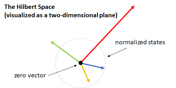
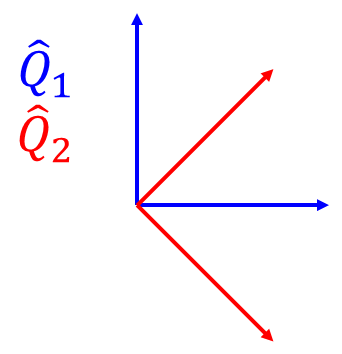
While the representation of the Hilbert space above as a two-dimensional plane is a pretty good visualization, it masks the fact that this is a complex vector space, whereas the plane is really a better representation of a real vector space. To make this more concrete, let’s call the normalized ket pointing to the right $\lvert0\rangle$ and the one pointing straight up $\lvert1\rangle$ . Then a vector that points up and to the right could look like

$\lvert\psi_0\rangle=\frac{1}{\sqrt{2}}\left( \lvert0\rangle + \lvert1\rangle \right)$

and one that points down and to the right is

$\lvert\psi_\pi\rangle=\frac{1}{\sqrt{2}}\left( \lvert0\rangle - \lvert1\rangle \right)$

However, it’s difficult to visualize, for example, the following state:

$\lvert\psi_{\frac{\pi}{2}}\rangle=\frac{1}{\sqrt{2}}\left( \lvert0\rangle + i\lvert1\rangle \right)$

In fact, in general, we could have states that look like this:

$\lvert\psi_\varphi\rangle=\frac{1}{\sqrt{2}}\left( \lvert0\rangle + e^{i\varphi}\lvert1\rangle \right)$

where $\varphi$ is called the relative phase. Note that $\varphi=0$ , $\varphi=\pi$ , and $\varphi=\frac{\pi}{2}$ correspond to the three cases above.

Suppose I wanted to measure whether the state is in state $\lvert1\rangle$ , which corresponds to the observable $\hat{Q}_1=\lvert1\rangle\langle1\rvert$ . Then the possible results are “yes” (1) and “no” (0). The former result corresponds to a projection $\hat{P}_{1,\lambda=1}=\lvert1\rangle\langle1\rvert$ and the latter corresponds to $\hat{P}_{1,\lambda=0}=\lvert0\rangle\langle0\rvert$ . Suppose we measure $\hat{Q}_1$ for the state $\lvert\psi_\varphi\rangle$ . The probability of measuring $1$ for this observable is

$P(\lambda=1)=|\hat{P}_{1,\lambda=1}\lvert\psi_\varphi\rangle|^2=|\lvert1\rangle\langle1\rvert\frac{1}{\sqrt{2}}\left( \lvert0\rangle + e^{i\varphi}\lvert1\rangle \right)|^2=|\frac{1}{\sqrt{2}}\left( \lvert1\rangle\langle1\rvert0\rangle + e^{i\varphi}\lvert1\rangle\langle1\rvert1\rangle \right)|^2=|\frac{1}{\sqrt{2}}\left( \lvert1\rangle\cdot0 + e^{i\varphi}\lvert1\rangle\cdot1 \right)|^2=\frac{1}{2}$

after which the state would collapse to state $\lvert1\rangle$ .

In a way, this state is an “equal superposition between $\lvert0\rangle$ and $\lvert1\rangle$ .” Oftentimes, especially in popular science, people talk as if there isn’t more to quantum than systems being in “between” two classically discrete states. The reality is clearly more nuanced than that. There is a probability of one half that we find this particular state in $\lvert1\rangle$ . However, notice that this doesn’t depend at all about the relative phase $\varphi$ . This begs the question of why we care about relative phase if it doesn’t seem to do anything here.

The answer is that the relative phase doesn’t affect the probability of measuring this particular observable. However, we can instead consider the observable corresponding to whether or not the state is in state $\lvert\psi_0\rangle=\frac{1}{\sqrt{2}}\left( \lvert0\rangle + \lvert1\rangle \right)$ . This corresponds to the operator $\hat{Q}_2=\frac{1}{2}\left( \lvert0\rangle + \lvert1\rangle \right)\left( \langle0\rvert + \langle1\rvert \right)$ . Now the projection operators we need for this observable are $\hat{P}_{2,\lambda=1}=\frac{1}{2}\left( \lvert0\rangle + \lvert1\rangle \right)\left( \langle0\rvert + \langle1\rvert \right)$ and $\hat{P}_{2,\lambda=0}=\frac{1}{2}\left( \lvert0\rangle - \lvert1\rangle \right)\left( \langle0\rvert - \langle1\rvert \right)$ . The probability of measuring that the state is in $\lvert0\rangle + \lvert1\rangle$ is

$P(\lambda=1)=|\hat{P}_{2,\lambda=1}\lvert\psi_\varphi\rangle|^2=|\frac{1}{2}\left( \lvert0\rangle + \lvert1\rangle \right)\left( \langle0\rvert + \langle1\rvert \right)\frac{1}{\sqrt{2}}\left( \lvert0\rangle + e^{i\varphi}\lvert1\rangle \right)|^2=|\frac{1}{2\sqrt{2}}\left(\lvert0\rangle\langle0\rvert + \lvert0\rangle\langle1\rvert + \lvert1\rangle\langle0\rvert + \lvert1\rangle\langle1\rvert\right)\left( \lvert0\rangle + e^{i\varphi}\lvert1\rangle \right)|^2=|\frac{1}{2\sqrt{2}}\left(\lvert0\rangle\langle0\rvert0\rangle + \lvert0\rangle\langle1\rvert0\rangle + \lvert1\rangle\langle0\rvert0\rangle + \lvert1\rangle\langle1\rvert0\rangle + e^{i\varphi}\lvert0\rangle\langle0\rvert1\rangle + e^{i\varphi}\lvert0\rangle\langle1\rvert1\rangle + e^{i\varphi}\lvert1\rangle\langle0\rvert1\rangle + e^{i\varphi}\lvert1\rangle\langle1\rvert1\rangle\right)|^2=|\frac{1}{2\sqrt{2}}\left((1 + e^{i\varphi})\lvert0\rangle + (1 + e^{i\varphi})\lvert1\rangle\right)|^2=\frac{1}{2} + \frac{1}{2}\cos\varphi$

after which the state would collapse to state $\lvert\psi_0\rangle$ .

We see that the probability of measuring the state $latex \lvert\psi_\varphi\rangle$ in state $\lvert\psi_0\rangle=\frac{1}{\sqrt{2}}\left( \lvert0\rangle + \lvert1\rangle \right)$ is $\frac{1}{2} + \frac{1}{2}\cos\varphi$ . Note that this is equal to $1$ when $\varphi=0$ , when $\lvert\psi_\varphi\rvert = \lvert\psi_0\rvert$ . It’s equal to $0$ when $\lvert\psi_\varphi\rvert = \lvert\psi_\pi\rvert$ , which is perpendicular to $\lvert\psi_0\rvert$ . Indeed, when we measure this second observable, called measuring in a different basis.

The basic gist of what would happen here is this: if I measure $\hat{Q}_1$ over and over again, no matter what the state started with, I will always measure the same thing. This is because the first measurement collapses the original state into an eigenstate (eigenvector) of the $\hat{Q}_1$ operator. However, if I measure $\hat{Q}_1$ , then $\hat{Q}_2$ , and $\hat{Q}_1$ again, I will actually only get a 50% chance of measuring the state in $\lvert1\rangle$ .

While a bit more nuanced, in quantum mechanics, a similar thing goes on with position and momentum. If you measure the position over and over again, you will get the same answer each time. However, if you measure the momentum, the state will collapse to an eigenstate of the momentum operator, and, if you measured the position again, it wouldn’t be in the exact place anymore. In fact, if you measured the momentum perfectly, it turns out that you lose all position information. This underlies Heisenberg’s uncertainty principle between position and momentum, which says that the product of the uncertainties for position and momentum $\sigma_x\sigma_p$ must be at least a nonzero constant $\frac{\hbar}{2}$ .

Now, this two-state system seems like a pretty abstract quantum system, but it’s actually not. Many systems are effectively two-state systems. This includes

The polarization of light
The spin of an electron
The energy level of an electron in an atom if only two levels are realistically likely

The two-state system is really important in quantum information and computation, the underlying idea of which is that the weirdness of quantum mechanics can be used to solve certain problems which cannot be efficiently solved by classical computers. By efficiently, I mean it would be nice to solve certain problems before the heat death of the universe trillions of years from now, but for some problems we actually can’t do that with classical computers. That’s not a really high bar for efficiency, but some problems, like factoring semiprime numbers (which is relevant for a security protocol called RSA) are really that hard.

The fundamental unit of these quantum computers is the quantum bit, usually abbreviated to qubit. Each qubit is a two-state system. If you consider $N$ qubits together, the Hilbert space spanned by all of them actually has dimension $2^N$ . For example, if I have two qubits, I can take the basis $\beta=\lbrace\lvert00\rangle,\lvert01\rangle,\lvert10\rangle,\lvert11\rangle\rbrace$ , which has four ( $2^2$ ) elements in it. This is often pitched as $N$ qubits being equivalent to $2^N$ classical bits, although the reality is, as always, a bit more nuanced than that.

Part 5: Going Further

I have covered here a basic overview of linear algebra and introductory quantum mechanics. Of course, if you want to be able to do any of these subjects, go beyond this summary and explore these beautiful subjects. In this section, I’m going to discuss some topics which are cool extensions of linear algebra and quantum mechanics.

Linear Algebra

Numerical linear algebra, which is the use of algorithms to do linear algebraic operations. Note that matrices are very important in computation because it turns out that, while, say, humans have a difficult time inverting matrices and stuff like that, computers are actually quite good at it. It’s also extensively used in subjects like machine learning.
Abstract algebra, which is a generalization of linear algebra (hence the “linear” part is replaced by “abstract”). One key object in abstract algebra is that of groups (the study of which is called group theory), which are this generalized algebraic structure which basically underlie the mathematical study of symmetries. Other objects in abstract algebra are rings (ring theory), which are specific kinds of groups or, if you would like, generalized fields (for example, the integers $\mathbb{Z}$ are not a field, but they are a ring), and modules, which are like vector spaces except, instead of being over a field, they only have to be over a ring.
Functional analysis, which is the study of special kinds of infinite-dimensional vector spaces.

Quantum Mechanics

Quantum information and computation, which, as stated before, is the use of quantum mechanical weirdness in building quantum computers, which could theoretically efficiently solve problems which we believe that classical computers cannot.
Quantum field theory (QFT), which describes all particles as perturbations in fields. In QFT, particle number is not necessarily conserved, and special relativity is fully accounted for. Quantum field theory is possibly the best tested theory in all of physics, predicting the g-factor of the electron to thirteen decimal places and the Hall conductance to nine. When applied to electromagnetism, this is called quantum electrodynamics (QED). When applied to the strong force, it’s called quantum chromodynamics (QCD). When applied to the weak force, it’s called quantum flavordynamics (QFD), although people often resort to the electroweak model for this.
Particle physics, the study of subatomic particles, which obey quantum mechanics. The current best accepted model of particle physics is the standard model, although we know that there are subtle some problems with it. There are also a lot of people trying to figure out how dark matter fits into all of this.
String theory, loop quantum gravity, and other theories of quantum gravity. We’re really off the deep end here.

Acknowledgements

The linear algebra presented here is inspired by material from the following courses at UC Berkeley:

Physics 89 (Austin Hedeman)
Math 110 (Zvezdelina Stankova)

The quantum mechanics presented here is inspired by material from the following courses:

Physics 5C (Mina Aganagic)
Physics 137A (Austin Hedeman)

For further reading on linear algebra, especially in physics, some texts I can point to are

Yes, I am not making those names up. This is actually what those books are called.

For further reading on quantum mechanics (and, believe me, if you want to actually know how to do quantum mechanics, you should read further), consider

Nicholas Rui

Linear Algebra and Quantum Mechanics

Part 1: The Abstract

Part 2: A Theory of Vector Spaces

Vector Addition Axioms:

Scalar Multiplication Axioms:

Distributive Axioms:

Some Loose Ends:

Linear Independence

Spanning and Bases

Linear Transformations

Eigenstuffs

Inner Products

Other Linear Transformation Definitions and Theorems

Part 3: The Quantum Mechanics—The Postulates

Part 4: The Two-State System

Part 5: Going Further

Linear Algebra

Quantum Mechanics

Acknowledgements

Leave a Reply Cancel reply

Part 1: The Abstract

Part 2: A Theory of Vector Spaces

Vector Addition Axioms:

Scalar Multiplication Axioms:

Distributive Axioms:

Some Loose Ends:

Linear Independence

Spanning and Bases

Linear Transformations

Eigenstuffs

Inner Products

Other Linear Transformation Definitions and Theorems

Part 3: The Quantum Mechanics—The Postulates

Part 4: The Two-State System

Part 5: Going Further

Linear Algebra

Quantum Mechanics

Acknowledgements

Share this:

Like this:

Leave a Reply Cancel reply